Hubble Space Telescope Image of 3C-273 – Credit: ESA/Hubble/NASA

I often get asked about how far the telescope in Raheny can actually see.  The answer is in theory infinity, but practiaclly there are limits.  In 2012 I made an observation of one of the most distant and exotic objects in the universe.  Measuring the distance to one of the brightest quasars would not be easy.  Here’s the story of how it happened.

Quasars are the super-luminous cores of very distant galaxies which are thought to surround a super-massive black hole.  Rather than give a dissertation on the nature of quasars, here is a link describing quasars generally and a specific link to 3C-273.  If you need to go and have a read and then come back to this page.

Instrumentation.

3C-273 has a visual magnitude of ~+12.9 meaning it would be right on the edge of visibility in amateur telescopes.  If you wish to view 3C-273 optically (an 8 inch telescope under a dark sky should easily do it) then see here for some detailed finder charts.  My equipment consists of a 14″ Schmidt-Cassegrain telescope on an Astro-Physics 1200GTO mount.  The spectrograph used is home built.  It consists of a 300 lines/mm optical grating and an adjustable slit to ‘sample’ the light from the target object, various optics then focus the light on a CCD camera (currently ATIK 4000).  The beauty of this spectrograph is the ability to capture the entire visible spectrum plus a lot of infrared and ultra violet on one frame of the camera.

One of the difficulties of spectroscopy is positioning the target object on this slit which is only about 30microns wide and then keeping it there as the telescope tracks across the sky.  The difficulty of this cannot be underestimated but having a tried and trusted workflow helps a lot.  There also needs to be some method of ‘autoguiding’ while imaging a spectrum.  Anyone who has tried ‘autoguiding’ knows it can be a non-trivial task in itself, now couple that with the exacting requirements of spectroscopy, specifically keeping a magnitude +12.9 star focused on a 30micron slit, and you can see the difficulty.

Imaging and Processing – 3C-273.

15 x 150 second exposures were taken.  The camera is binned 2×2.  This gives me a theoretical resolution of 4 angstroms per pixel.  This resolution can be increased to 2angstroms/pixel by binning 1×1 however an object like 3C-273 does not require this sort of resolution.  After collection of the raw images, calibration frames (neon reference spectra and dark frames) are taken.  Given that these images are taken in a urban location, light pollution becomes a huge problem.  Fig 1.1 below shows a raw image from the camera (Uncalibrated).  The horizontal line is the spectrum of 3C-273, the vertical lines are caused by elements such as sodium (street lights) and other forms of light pollution.  I will describe my process for removing this.  The simple ‘cure’ is to subtract a section of the image which only contains light pollution from the section containing the spectrum, in theory this should leave only the spectrum behind and no light pollution.  While this does a great job of removing light pollution, some of the spectrum data is also lost resulting in a diminished signal/noise ratio.  Therefore it is vital to get a good signal to begin so that a useable image remains after the light pollution has been removed.

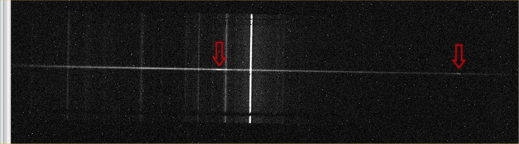
Fig 1.1 – Raw unprocessed fram showing the spectrum of 3C-273 (horizontal) and light pollution (vertical)

So to begin all the images are dark frame subtracted and then stacked together to produce an image with a strong signal/noise ratio. Some adjustments are made to ensure the spectrum is perfectly vertical in the image.  Next the image is processed to remove the light pollution (described above), with all that done we can then begin the real work of turn this streak of light into something meaningful.  The processed image is opened using Visual Spec, a wonderful piece of software written by Valerie Desnoux and made freely available for download.  VSpec turns this streak of light ito a graphic which illustrates the intensities recorded across the spectrum.  Obvious are two peaks visible (arrowed red in Fig 1.1) the one were interested in is the one on the right for reasons which will be shortly explained.  After producing the graphic in VSpec the next thing to do is to correct the graphic for the fact that CCD detectors respond to varying wavelengths of light in a  non linear fashion.  With this process completes we can now start to analyse the spectrum.

Analysis

Fig 1.2 Calibrated spectrum of 3C-273

So what is this bright spot on the right hand side anyway and what does it tell us.  Well examining the graphic above we can see that the peak of this ‘brightspot’ or ’emission line’ as it more correctly called is centred at 7568 angstroms.  From previous research we know that this is in fact the Hydrogen-Alpha emission line which is normally found at 6563angstroms.  So what is it doing at 7568angstroms?  The answer lies in the nature of the universe.  Most of us know that the universe is expanding and that everything in it appears to move away from every other thing.  We also take into account a phenomenon known as the ‘doppler’ effect.  When a wave of light (or sound) is moving towards us its wavelength gets compressed and becomes shorter (more blue) as an object moves away from us its wavelength gets longer (more red).  This is the same effect we hear as a police siren passes, the sound get higher pitched as the car moves towards us and starts to fall as the vehicle moves away.  Also as the light travels across the universe, space itself is expanding and thus the wavelength of the light is stretched even further.  The net result is that although the light had a wavelength of 6563angstroms when it left the object (as observed by a nearby static observer) the factors above ensure that the wavelength of light we see is much longer indeed.

From this we can measure a very special number for any object, its redshift or simply ‘z’.  The following formula tells us what the redshift for 3C-273 is.

z = (Measured Wavelength/Static Wavelength) – 1  in this case z = (7568 / 6563) – 1 = .153.  Viola, a result!  This is very much in keeping with the published z value of 3C-273 of .158.  (Thanks to David Haworth for pointing out a typo here)  So z=.153, big deal, what can this tell us?  Well the good news is that there is a relationship between z and distance to the object.

D_o = z * C /h where C is the speed of light in a vacuum and h is a very special value known as the ‘Hubble constant’ (read about it if you like).  The interesting thing of note about h is that in fact although in theory it is a constant, in practice you will find many different answers as to its value.  Depending on who you ask you will find an answer somewhere in the range 65 – 78 kms/sec per mega parsec.  So lets split the difference and call it 72 kms/sec. and fill this in and we get.

D_o = .158 * 30000000 / 75 = 632,000 mega parsecs.  Given that 1 parsec = 3.26156 light years we can conclude the distance to 3C-273 as 2,061,305,920 light years or 2.06 billion light years!

Not bad for a home built spectrograph eh?

Observation Time 15th April 2012 – 00:00 – 02:00 UT